Been busy
In part due to this guy… be back soon…
In part due to this guy… be back soon…
The bridge that carries Route 381 over the Youghiogheny River has been there a fairly long time. At least in some form or another. We have often wondered if the placement of the piers have affected the river scour at this site, as there is a downward trend in the habitat quality at this particular site. The pier is directly in front of the scour and may deflect the following water from directly hitting the scour.

A bridge pier in front of the a river scour. The Youghiogheny is flowing from the right to the left.

The other side of the bridge pier from the previous photo.
Just downstream of here, one can see a lot of the grasses are bent in the upstream direction, indicating that there’s some sort of eddy operating here. I’ve seen similar eddys at the downstream end of river scours before, typically after a series of rapids.
So many interesting questions about scour hydrology!

My friend Lisa Smith, executive director of the Natural Areas Association convinced me to buy this book, The Future of Conservation in America: A Chart for Rough Water, at the NAA table at the Pennsylvania Botany Symposium. The authors, Jonathan Jarvis and Gary Machlis, delivered the closing plenary based on this book at the 2018 NAA Conference (I had to unfortunately miss it due to the Northeast Natural Heritage meeting scheduled at the same time). Unfortunately, this sat on the back of my couch for far too long before getting a chance to read it over the holiday break.
In short, this is a great short book. The authors, with decades of experience in the conservation field, are well qualified to cover this topic. They skillfully weave the core contributions of land protection and conservation science with the social, economic, and political facets of conservation. Speaking of politics, this book doesn’t shy away from the politics that affect land and water protection. As I write this, the federal government is in day seven of a shutdown over funding for Trump’s ecologically destructive (and frankly ridiculous) border wall. The authors don’t fail to recall that the previous long government shutdown was ended in part of by access to our national parks:
… the sixteen-day federal government shutdown in 2013 became an exercise in political theater, diversion of administrative effort, and economic disruption. The public outcry over the closure of parks ultimately forced the hand of Congress but reaffirmed the strong position that public lands have in American society.
(page 27)
They make the case that conservation in the future may be impeded by the lack of public support for science, especially as it relates to climate change.
Additionally, I was pleased to see a small shout-out to NatureServe and its Network of Natural Heritage Programs:
“Nonprofit organizations like The Nature Conservancy or NatureServe maintain their own research staffs…”
(page 74)
Natural Heritage data has a role in almost every natural area conservation decision in the US, and its unfortunately frequently unappreciated as part of the process. It’s good to see it referenced here.
This book is a great short read and has an inspiring message to an issue that seems dark at times. Highly recommended.
This book is available directly through the publisher or probably can be ordered through your favorite bookseller.
ps. A video of Machlis and Jarvis’ talk at the NAA meeting can be found here. Check it out after you read the book, or before, or even if you don’t read this book.
As I've gotten more active on science Twitter after a long absence, I recently become more aware of the #365papers thing. Digging into it, it seems like something I would be into: reading papers, sharing them, setting unrealistic goals...
I'm going to set some rules:
I'll update a list of the papers read here below.
Recently, I’ve been beginning to dabble in 3D GIS, something I have very little experience with. Co-incidentally, on a recent trip through Ontario, I came across this incredible example of a 3D mine map. Each map “sheet” was printed on plexiglass, and stored in a custom cabinet, lit from below, so they are below so the structure and relationships between the levels of the mine could be examined. A pretty great example of 3D mapping before it was commonplace.

A 3D map of a mine (at the Bancroft Mineral Museum)

from https://github.com/zonination/perceptions
I'm currently working on a project where we are presenting information on the possible presence of particular species at sites across the state. We're considering the fairly ordinary words of 'high', 'medium', and 'low' to describe the probability, These words, of course, can connote a particular meaning to the users of this analysis. In order to make a decision on which words to use, we're beginning to look at the mean behind commonly used phrases.
This great work, by redditor zonation, provides of some great examples of what a surveys mean. This is based on Sherman Kent's work in the 1960's. Its definately provides a great framework to understand how people may understand our data presentation.

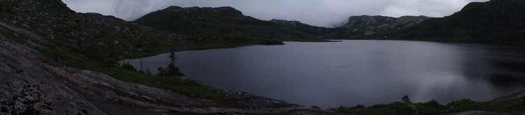
An icy Youghiogheny River at Ohiopyle, Pennsylvania (January 2018).
One of my favorite plant communities are Floodplain Scours -- areas of relative bare rock that occur along the banks of major rivers where rock outcrops are subject to winter ice scour and high-velocity flooding. Along the Youghiogheny River in Fayette County, PA these communities occur along bedrock shelves and boulders. The ice and flooding removes competition from many plant species allowing a number of threatened and endangered species such as rock grape (Vitis rupestris), Carolina tassel-rue (Trautvetteria caroliniensis) and large-flowered Barbara's buttons (Marshallia grandiflora) to survive.
Last weekend, my colleague Pete Woods and I went down to the Yough to check out these scour zones during ice conditions as we figured it would be a good time to check out the ice conditions as this region of the country had been in a multiweek deep freeze. In fact, the thermometer on the car read as low as -15F on the way down (it did warm up to nearly 20F by the time we left shortly after lunch.

A large chunk of ice resting on the scour zone.

Remains of last year's Large Flowered Barbara’s-buttons (Marshallia grandiflora) along the Youghiogheny's scour zone.
Floodplain Scour communities are most likely declining due to destruction of plant populations and the alteration of ecosystem processes needed to maintain these populations. Alteration of the natural flooding regimes through construction of dams and other impoundments has greatly impacted the plant composition. As the amount and frequency of flooding and ice-scour are the most critical factors maintaining the quality and persistence of this community, factors that can change these attributes such as the effects of global climate change is the potential loss of ice scour as the climate warms.

Even in the middle of winter, we found some lichens to collect. This particular rock is fairly inaccessible during the growing season, so it was interesting to look at up close.

We're a little over a week away from the opening of Star Wars: The Last Jedi, the latest installment in the Star Wars franchise. While I've been diligently avoiding any major spoilers for the film, its been hard to miss the mania around Porgs--one of the new creatures that will make their debut in this movie.
As a portion of the movie was shot on the Irish island of Skellig Michael, providing the location of the planet -- where Luke Skywalker spent many years in exile before he was found at the end of Star Wars: The Force Awakens, one of the challenges the filmmakers had to deal with was the abundant seabird colonies. Species using the island for breeding habitat include the Atlantic Puffins (Fratercula arctica), Fulmars (Fulmarus glacialis), Arctic Terns (Sterna paradisaea), and Northern Gannets (Morus bassanus). Apparently, birds were frequently seen in the background of shots. Rather than trying to digitally remove them, they decided to go all in and use them as (minor???) characters in the film, now known as Porgs.
Based on the relatively scarce information released on them, Porgs appear to be based on the puffin, however, at least to my eyes, they cross taxonomic classes and have the face of an otter. Rian Johnson, the movie's director put out some additional details in a tweet a while back:
They are sea birds. Their coloring varies. Males are slightly larger than females. They can fly short distances. They're inquisitive.
— Rian Johnson (@rianjohnson) September 13, 2017
The young are also apparently called porglets. I'm a little skeptical that they can fly well based on the size of their wings, but aerodynamics are one thing that don't always make sense in Star Wars. This short animation Disney put out over the summer shows that they are also a gregarious species and they appear to be as clumsy on the ground as their inspiration, the puffin. From this clip, as well as a brief appearance in a trailer, it seems Porgs can vocalize, while their real-life counterparts are silent except for a chainsaw-like growl when they are in their burrows.
One of the interesting things about this are the ecological impacts of filming at this location, as it is an important breeding site for puffins and the other seabirds that call the site home as well as a UNESCO World Heritage site. Apparently there was some controversy from the filming during the relatively short amount of time the island was in the The Force Awakens, as some of the bird species were still breeding at the site and disturbed by the activity. Additional precautions and measures were put in place for the sequel, but the long term effects of the use of the site are unknown at this time. An additional complicating influence will be increased tourism to the site, something the Irish government hopes island’s film appearance will help bring.

Alpine-azalea (Kalmia procumbens) in fruit.
One of the highlights of the botanical finds I had during this past trip to Newfoundland was the Alpine-azalea (Kalmia procumbens). This small shrub is a member of the Ericaceae that forms a cushion-like mound about 10 centimeters (4 inches) tall. Inhabiting northern, alpine regions around the world, it has tiny pink flowers tucked in between the leathery, opposite leaves. Like many of the plants I had wanted to see, I had missed this species in flower, but the fruits were just as cool.
The compact growth form is known in botanical circles as a "cushion plant" growth form is found in alpine habitats across the world and across a number of plant families. These are actually masses of individual stems that grow very slowly and at the same rate so one stem is not more exposed than then another. This allows the plants to survive cold and harsh climates. Additionally, its tough leaf cuticles protect it from the cold winds that can dessicate the plants.
More details about this species can be found on Go Botany.

Habitat for alpine azalea at Mistaken Point Ecological Reserve.
Today, I stopped by the aptly named Fringed Gentian Fen a small piece of protected wetland just north of Pittsburgh. One of the highlights of this site is a good sized population of Fringed Gentian (Gentianopsis crinita).

Gentianopsis crinita
This species is only found in a few scattered locations in western Pennsylvania, whereas it's a little more abundant in the eastern part of the state. It's usually found in richer, open wetlands, although I've also seen it along stream banks in Erie County. It's truly one of the most striking wildflowers in the region.

This species is the inspiration behind one of William Cullen Gentian's poems.
To the Fringed Gentian
Thou blossom bright with autumn dew,
And colored with the heaven’s own blue,
That openest when the quiet light
Succeeds the keen and frosty night.
Thou comest not when violets lean
O’er wandering brooks and springs unseen,
Or columbines, in purple dressed,
Nod o’er the ground-bird’s hidden nest.
Thou waitest late and com’st alone,
When woods are bare and birds are flown,
And frosts and shortening days portend
The aged year is near his end.
Then doth thy sweet and quiet eye
Look through its fringes to the sky,
Blue-blue-as if that sky let fall
A flower from its cerulean wall.
I would that thus, when I shall see
The hour of death draw near to me,
Hope, blossoming within my heart,
May look to heaven as I depart.

Outside of ecology and conservation, one of the things that I am really into is Star Wars. A few months ago, Rogue One, the first anthology film in the Star Wars universe was released. This was preceded by a tie-in novel, Catalyst, that is a prequel to the the movie. The events in the book take place from the somewhere before the events portrayed in Star Wars: Episode III – Revenge of the Sith to immediately prior to the events of the 2016 Star Wars Anthology film Rogue One.
Note: spoilers for both the book and the movie follow, so proceed at your own risk.
As even the most casual fan of Star Wars knows, the Death Star is the size of a "small moon". A space station of this size would have to take an amazing amount of raw materials to build. I often wondered about the resources it would take to build such a station, not to mention the all the other ships of the Empire and the Rebel Alliance.
The Catalyst novel covers some of the exploitation of these resources during the two decades before the Battle of Yavin. As the Death Star is the the signature of the Empire, they are in a ruthless in its pursuit of the incredible amount of natural resources. While many planets were open to resource extraction, they also introduced the concept of a "Legacy World"--a term for planets that were environmentally-protected and legally exempted from exploitation. Limited industrial presences on this world were regulated so to be low-impact. The Empire finds ways to override environmental protections on these Legacy Worlds. When the Empire cannot simply claim these protected resources for themselves, they trump up falsehoods as justification for annexing resource-rich planets and taking what they need. In the end many planets are devastated by the Death Star project.
While reading this book, I could help to see the parallels between story and current efforts by some facets of Federal and state governments, corporations, and other parties to reduce or eliminate environmental protections on publicly owned land in the US, largely in the name of economic development. While it was a little stressful to read a book for entertainment that so strongly reminded me of work, it was good to see this issue covered in (semi-)popular media. So much for escapism though...
During my last visit to Newfoundland, my friend Emma and I made a ridiculous journey from across Newfoundland and back over the course of about 30 hours, all in the idea of seeing puffins. One of the folks that we met on the Long Range Traverse mentioned this great place on the east coast, where one could view a puffin colony from land. Intrigued, we drove to Elliston, NL to see some Atlantic Puffins (Fratercula arctica) --a first for both of us. It was a short trip, but well worth it.
On this recent return trip that Martha, Ellery, and I recently took, one of our must-see stops was a revisit to Elliston, so Ellery could see her second-favorite seabird. Leaving Gander early on a Sunday morning, we stopped for a few hours on our way towards St. John's. The puffin viewing on this visit was amazing. One of the fascinating things about this site, is that the island that the puffin colony is on is only about 150 meters from mainland. Its probably the closest that one can view these birds where one doesn't have to be on a boat. The morning we visited had puffins hanging out on the mainland, many of them only a few meters from where we were sitting.

The flower of Opuntia cespitosa. Notice the red-orange bases of the tepals, compared to the pure yellow flowers of O. humifusa.
A few weekends ago, I was messing around on Facebook, when a blog post by the New England Wildflower Society caught my eye. This article highlighted a split in of the eastern prickly pear cactus (Opuntia humifusa) into two species--O. humifusa and O. cespitosa. I shared it with our botanist at work, and he agreed that it appeared to be a valid taxonomic split, supported by a variety of methods. It's interesting that O. cespitosa is an originally a name given by Rafinesque in the 1800s. Like, many of the species Rafinesque described, there was no type species available and, over time, the species was lumped into O. humifusa. The recent work that led to the resurrection of this species was done by Lucas Majure (papers linked from here).
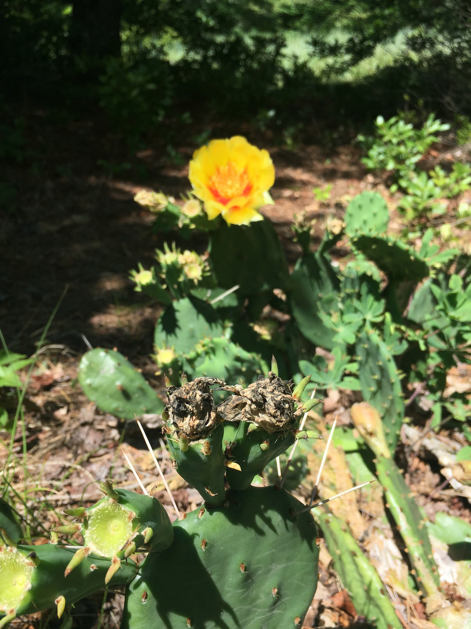
Notice the long spines on the pads, this is one of the features that differentiated this species from Opuntia humifusa.
Looking around in the online herbarium databases (the benefits of digitized collections), we found a putative example of this species in Pennsylvania from an 1862 specimen along the Susquehanna River. Not being aware of any extant populations, we were planning on ending this to the Pennsylvania flora as an extirpated species.
However, I was up in Erie County working on vegetation plots, when we came across a small population of Opuntia that I had documented a few years previously. Back then, I had called it O. humifusa, as I wasn't aware of another taxon in the state at the time. However, this time the species was in flower, and it was obvious from that this was indeed O. cepitosa given the red-orange coloration of the flower and the long spines. This was a fairly exciting change in identity for this population of the species, especially as we now have a confirmed extant population of this species in Pennsylvania.
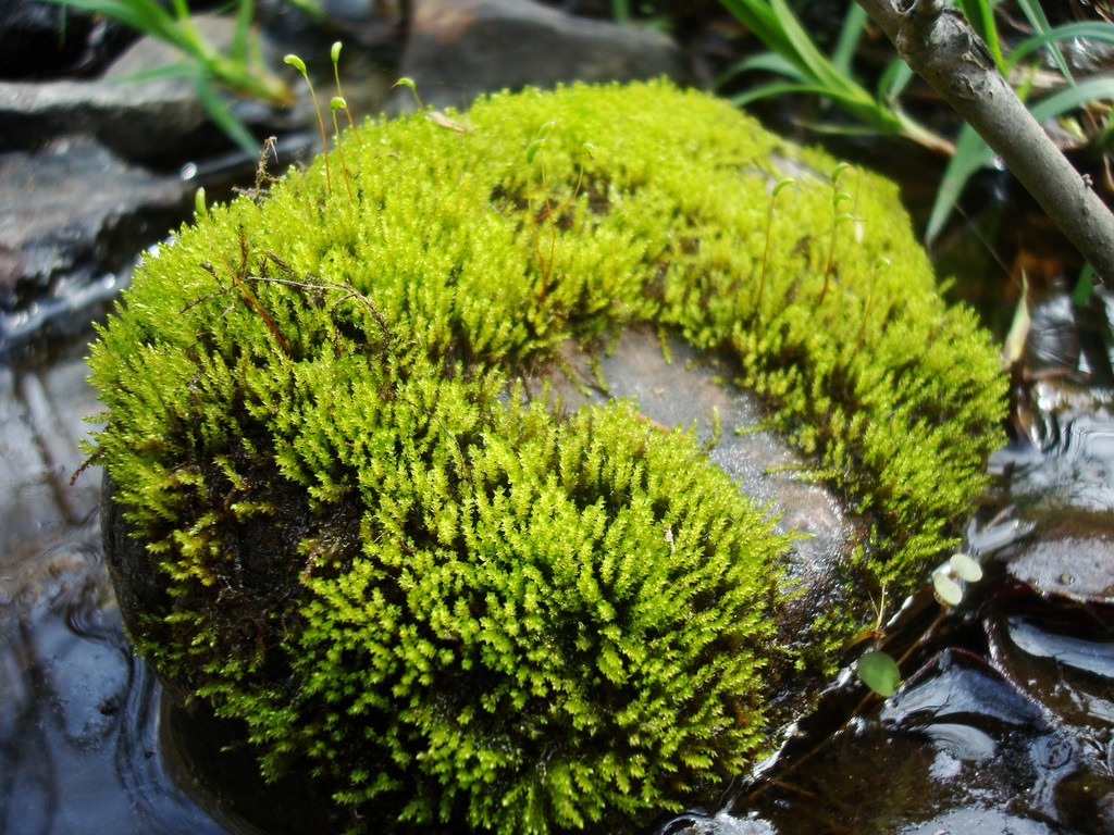
My colleague Scott Schuette and I recently published an updated checklist of the bryophytes (mosses, liverworts, and hornworts) of Erie County, Pennsylvania. We began this project back in 2012, when Scott was asked to help arrange for the annual Crum Workshop (a regional bryophyte foray) to be hosted somewhere in Pennsylvania. We were just in the process of wrapping up the update to the Erie County Natural Heritage Inventory--so we thought that would a great location to host the workshop. Through this five-day gathering of bryologists and additional inventory through heritage survey work, we increased the known number of bryophyte species in the county from 82 to 199, with eight species reported for the first time in Pennsylvania. More details in the abstract:
One hundred ninety-nine species of bryophytes are documented for Erie County, Pennsylvania, representing 34% of the Pennsylvania bryophyte flora. This work is the result of scattered surveys over multiple years and the 2012 Crum Workshop. Aneura maxima, Calypogeia integristipula, C. sphagnicola, Fuscocephaloziopsis loitlesbergeri, F. macrostachya, F. pleniceps, Cephaloziella hyalina, and Campylium protensum are reported new to the state, and an 83 species are reported new for the county. Nearly 40% of the species on this list are considered “rare” and tracked as critically imperiled (S1), imperiled (S2), or vulnerable (S3) by Pennsylvania Natural Heritage Program, highlighting the critical role of intensive surveys for bryophyte conservation.
For those interested in reading the full article, and have library access, here is the link on BioOne. Also, the Crum Workshop will be hosted in Pennsylvania again this year. It will be held in the State College area and we'll again be visiting several different habitats for bryophyte inventory.
I've been really lax in writing about this amazing trip. About two years ago, I was looking for an interesting backpacking trip to do and I discovered a brief mention of a hike Gros Morne National Park in Newfoundland, Canada called the Long Range Traverse. The description was pretty brief, but I dug into the trip and I became really obsessed with trying it out. A chance run-in with a friend where I asked her if she wanted to go on a "ridiculous backpacking trip to Canada" resulted in a few months of preparation and planning.
After a mandatory park orientation including a backcountry navigation test and a humorously dated video, we spent the remainder of the day getting last minute supplies. Early the next morning, we dropped or rental car off at the end of the trail, where we had a taxi scheduled to drive us the 20 kilometers to the trailhead at Western Brook Pond. From here we had about a 45 minute walk to the end of a freshwater fjord, where we boarded a boat with two other groups of hikers as well as a number of tourists just there for the ride. The boat dropped us off at a small boat dock, where we got our gear ready and began the Long Range Traverse.
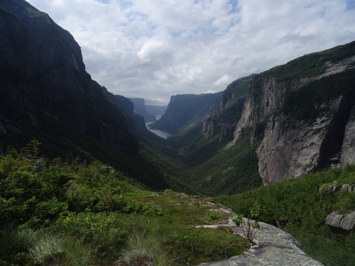
The top of the climb out of Western Brook Pond
Although they recommend solid map-and-compass skills for the trip, the first section up the glacial carved valley of Western Brook Pond is fairly straight-forward due to a well-worn trail and the presence of a few trail markers on trees--the latter betraying the statement that there are no trail markers along the 32-kilometer route. At the top of the 600-meter (~2000-feet) climb, including a near vertical climb next to a waterfall out of the valley, one is greeted by this amazing view! Additionally, the top of the gorge offers the first look at what you’re in for: a endless landscape of mountain meadows, rolling peaks, and shimmering lakes. Although striking, it is a slightly sobering expanse of wilderness --and one can’t help but note that everything sort of looks alike.
From here, navigation was a lot more difficult. Now we were above the treeline, where the harsh, icy winds have scoured the glacier-carved landscape. The trail of previous hikers more or less disappear and its easy to get lost via a navigation puzzle as you try to get around pockets of peatland and open water. Additionally, the meandering footpaths of caribou can entice you away from the proper course--which happened more than once to us. Of course, throughout the trip, there were numerous ecological side trips as I ditched the plan route to look an interesting bog or rock or followed a butterfly for perhaps far too long.
Fog rolling in
Although, we had great weather to see the view from the top of Western Brook Pond, fog was quickly rolling in that afternoon so we made some haste in heading toward camp, especially as we were getting our navigation skills up to speed.

While the whole Long Range Traverse is backcountry hiking and camping, five recommended camping areas with tent platforms and pit toilets are spaced throughout the area. The first night we camped at Little Island Pond. The pond did indeed have an island in the middle of it, which did look like an enticing place to explore via a swim, but the 10C water quickly killed that plan. Overall, this first leg of the trip felt relatively easy, at least easier than I imagined. The next few days would test that...
But we did wake up to this amazing view the next morning.

One common analysis in ecology and conservation planning is to divide the landscape up in regular units for sampling, reserve design, or the summarization of a variable. While squares are a common and easy way to divide the landscape, they are not the only way to divide the landscape up in regular units--hexagons being the other main choice. Birch et al. (2007) examined the use of hexagonal grids in ecological studies and concluded that there are benefits for representing movement and ecological flow as well as potentially providing better data visualization. They did note that hexagonal grids were rarely used, but its likely that their use has increased since their publication due to increases in computer power.
Regular hexagons are the closest shape to a circle that can be used for the regular tessellation of a plane. This give rise to the following benefits:
However, there are still some advantages of square grids compared to hexagon grids:
For a site-level conservation planning project that I'm currently working on, we had to develop a relatively small scale hexagon grid to prioritize conservation actions. One question we had to grapple with was the size of the hexagon, especially as it relates to usefulness and performance.To that end we began with examining the potential sizes of planning units we could create. Just for reference, we considered the 30-meter pixel as in many ways in the minimum unit of data that is available to us as its what many landcover and elevation maps are created at. Beyond that we considered 1, 5, 10, and 50 acre hexagons. Below is table of the number of planning units in Pennsylvania for each of the sizes.
| Area / Shape | ~ units in Pennsylvania |
|---|---|
| 30m square pixel | 300,000,000 |
| 1 acre hexagon* | 30,435,389 |
| 5 acre hexagon | 5,901,730 |
| 10 acre hexagon | 2,952,264 |
| 50 acre hexagon | 591,583 |
* = estimated, haven’t been able to run for the whole state
We had a number of discussions about this with our project partners and committee members. We immediately threw out the 900m2 size as there are about 300 million of them in the state and the computational needs would be immense--not to mention accuracy issues between the datasets. From some data gathered during some tests, as well as feedback about the scale that many users will be working out at, we've selected 10 acres as the size of the hexagon to work at.
Finally, for our use in this project one of the potential benefits is that hexagons allow patterns in the habitat data might be seen more easily than what squares cells may show.
Of course, being in Pennsylvania, I would love it if we could use these polygons!

A lot of the content in this post was inspired by this StackExchange discussion and this post by Matthew Strimas-Mackey. The latter also includes some great code for developing a hexagon layer. Additional code available in the dggridR R package.

A restored section of the mainstem of Nine Mile Run, Pittsburgh, PA.
I've been a member of the monitoring committee for the Nine Mile Run Watershed restoration for a number of years. The goal of the project, managed by the Nine Mile Run Watershed Association, is to accurately assess the health of Nine Mile Run, to help us understand what has been achieved and what remains to be done to reach a healthy ecosystem.
The committee recently completed a report card outlining the current progress of the restoration.
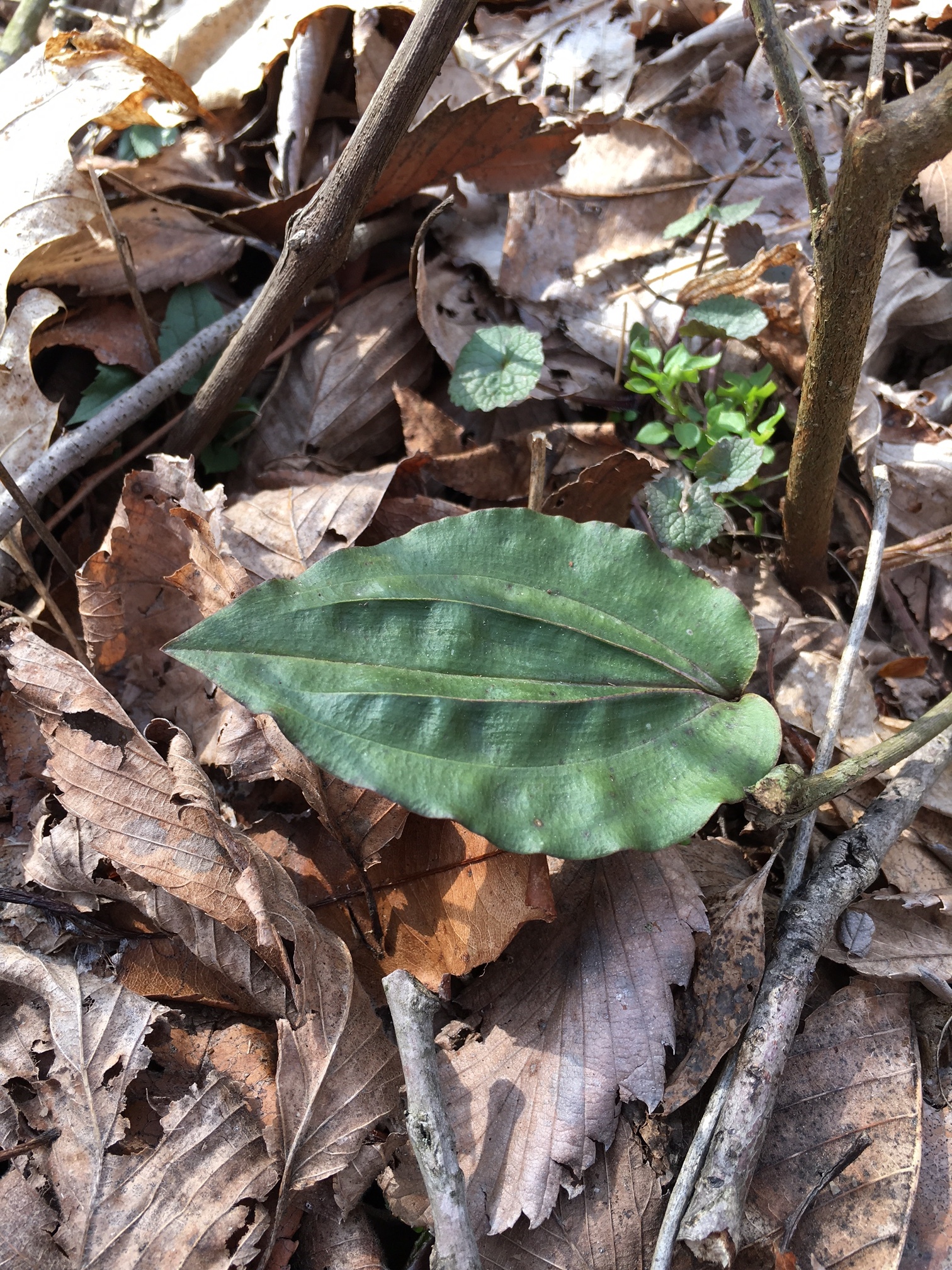
This past weekend, I spent some time volunteering on an ecological restoration project just south of Pittsburgh, PA. The goal of this project is to create habitat for forest birds through the removal of invasive shrubs such as Japanese barberry (Berberis thunbergii) and multiflora rose (Rosa multiflora) and to replace them with native shrubs. During the work, I happened to glance down and a unique leaf happened to catch my eye--the leaf of the Cranefly Orchid (Tipularia discolor)!
This particular site is fairly degraded and it was quite the surprise to find one growing here. I searched around some more and only found this one plant. There was a second leaf next to this one that had been ripped off--perhaps from trampling by one of the volunteers. This species is considered a watchlist species in Pennsylvania and one that we currently track through the Pennsylvania Natural Heritage Program.
The In Defense of Plants blog has a great post about the ecology and pollination biology of the species.
I've been working with my friend Steve Mather for a while now on setting up an analysis of forest structure across Pennsylvania and Ohio using LiDAR data. Our work has been slow-going.
As a concurrent project, I've been exploring a similar analysis in R in order to think more about the question and come up with an analysis framework for undertaking the work. I recently came across the excellent 'lidr' package for R that allows one for analysis LiDAR data for forestry applications. Having a small amount of extra time available the other night, I decided to dive in and explore some of the data.

Photo by Tim Ebbs / Flickr, CC
We're really interesting in comparing the forest structure as measured by LiDAR to field measurements by ecologists. Effectively, can we take a slice through the point cloud and extract a vertical column. Our current plots record information across the forest strata: 0-0.5m, 0.5-1m. 1-2m, 2-5m, 5-10m, 10-15m, 15-20m, 20-35m, and >35m.
Each of the Pennsylvania LiDAR tiles covers is four kilometers to a side and thus the file size is usually about 350mb per tile. We have about 13,500 of them in the state, so we're only working with one for this test and we'll scale up later. It was relatively straightforward to load a single LAS file into R using lidR.
lidar = readLAS("50001990PAN.las")Next, I generated a digital terrain model (DTM):
dtm = grid_terrain(lidar, res = 10, method = "knnidw", k = 6L)
This was a pretty quick proof-of-concept so the parameters for interpolating the grid are just placeholders. However, in later versions of this, we'll be able to use the DEM created by Pennsylvania TopoGeo as part of the original LiDAR collection.
The next step was to create a normalized point cloud that removes the ground contours and leaves us with just the canopy heights.
lidar_norm = lidar - dtm
From here, the next step was to calculate point density in each of the strata layers we measured in the field. First, we pulled out a slice of the point cloud (here's the zero to half meter extract:
ht0_0.5m = lidar_norm %>% lasfilter(Z>0.33,Z<1.64)
Then we calculate the point density:
den0m_0.5m <- grid_density(ht0_0.5m, res=5)
Here's a plot of the density for eight strata l

The next step is now to figure out how to summarize the point could density in each slice of the layer cake.

A quick little post for International Women's Day. My coworker Scott Schuette and I were recently working on a checklist of the mosses of Erie County, PA and a number of the specimens we included were from a women named Nelle Ammons who worked in the region in the first half of the 1900s. I've become fairly fascinated with her and have spent some of my spare time researching her story. There's terribly little biographical information written about her and most of what I found was in the History of Botany in West Virginia book, coincidentally written by spouse's great-uncle.
Nelle was born on 1889 in Greene County, PA and did undergraduate and master's work at WVU and then got her PhD from Pitt. She then ended up as an instructor at WVU and spent nearly 40 years there retiring as a botany professor in 1959. She did a pretty amazing amount of botany work in the region and authored a number of papers and books. I hope to dig more into her background in the near future.