Hexagons

One common analysis in ecology and conservation planning is to divide the landscape up in regular units for sampling, reserve design, or the summarization of a variable. While squares are a common and easy way to divide the landscape, they are not the only way to divide the landscape up in regular units--hexagons being the other main choice. Birch et al. (2007) examined the use of hexagonal grids in ecological studies and concluded that there are benefits for representing movement and ecological flow as well as potentially providing better data visualization. They did note that hexagonal grids were rarely used, but its likely that their use has increased since their publication due to increases in computer power.

Square versus Hexagonal grids

Regular hexagons are the closest shape to a circle that can be used for the regular tessellation of a plane. This give rise to the following benefits:

• A hexagonal grid gives the lowest perimeter to area ratio of any regular tessellation--this means that hexagons are effectively the are the best approximation of a circle that can be tessellated. In practice, as it relates to ecology, this means that edge effects are minimized when working with hexagonal grids.
• It may not be obvious that square grids have two classes of neighbors: 1) those in the cardinal directions that share an edge and 2) those in diagonal directions that share a vertex. In contrast, a hexagonal grid cell has six identical neighboring cells, each shares one of the six equal length sides. Furthermore, the distance between centroids is the same for all neighbors, compared to a square where where are two distances between cell centers.
• It is difficult to fit a square grid to the curved surface of the earth. Accounting for the curvature of the earth becomes increasingly important when working in large areas.

However, there are still some advantages of square grids compared to hexagon grids:

• The relationship between the each of the square cells is known based on distance and adjacency between cells.
• Combining raster layers is simple--algebraic operations combining multiple raster layers built on the same grid template simplifies to matrix algebra; no complex spatial operations are required.
• With squares there is an ease of resampling to different spatial scales; decreasing the spatial resolution only requires combining groups of four cells into one, whereas the spatial resolution can be increased by dividing each cell into four.

For a site-level conservation planning project that I'm currently working on, we had to develop a relatively small scale hexagon grid to prioritize conservation actions.  One question we had to grapple with was the size of the hexagon, especially as it relates to usefulness and performance.To that end we began with examining the potential sizes of planning units we could create.  Just for reference, we considered the 30-meter pixel as in many ways in the minimum unit of data that is available to us as its what many landcover and elevation maps are created at. Beyond that we considered 1, 5, 10, and 50 acre hexagons. Below is table of the number of planning units in Pennsylvania for each of the sizes.

Area / Shape	~ units in Pennsylvania
30m square pixel	300,000,000
1 acre hexagon*	30,435,389
5 acre hexagon	5,901,730
10 acre hexagon	2,952,264
50 acre hexagon	591,583

* = estimated, haven’t been able to run for the whole state

We had a number of discussions about this with our project partners and committee members. We immediately threw out the 900m2 size as there are about 300 million of them in the state and the computational needs would be immense--not to mention accuracy issues between the datasets. From some data gathered during some tests, as well as feedback about the scale that many users will be working out at, we've selected 10 acres as the size of the hexagon to work at.

Finally, for our use in this project  one of the potential benefits is that hexagons allow patterns in the habitat data might be seen more easily than what squares cells may show.

Of course, being in Pennsylvania, I would love it if we could use these polygons!

A lot of the content in this post was  inspired by this StackExchange discussion and this post by Matthew Strimas-Mackey. The latter also includes some great code for developing a hexagon layer. Additional code available in the dggridR R package.

Monitoring Nine Mile Run

A restored section of the mainstem of Nine Mile Run, Pittsburgh, PA.

I've been a member of the monitoring committee for the Nine Mile Run Watershed restoration for a number of years. The goal of the  project, managed by the Nine Mile Run Watershed Association, is to accurately assess the health of Nine Mile Run, to help us understand what has been achieved and what remains to be done to reach a healthy ecosystem. 

The committee recently completed a report card outlining the current progress of the restoration.

An Unexpected Discovery

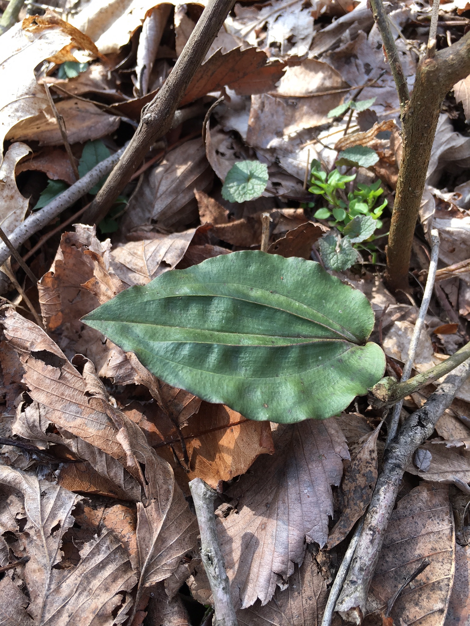
This past weekend, I spent some time volunteering on an ecological restoration project just south of Pittsburgh, PA. The goal of this project is to create habitat for forest birds through the removal of invasive shrubs such as Japanese barberry (Berberis thunbergii) and multiflora rose (Rosa multiflora) and to replace them with native shrubs. During the work, I happened to glance down and a unique leaf happened to catch my eye--the leaf of the Cranefly Orchid (Tipularia discolor)!

This particular site is fairly degraded and it was quite the surprise to find one growing here. I searched around some more and only found this one plant. There was a second leaf next to this one that had been ripped off--perhaps from trampling by one of the volunteers. This species is considered a watchlist species in Pennsylvania and one that we currently track through the Pennsylvania Natural Heritage Program. 

The In Defense of Plants blog has a great post about the ecology and pollination biology of the species.

LiDAR and Forests: Part 1

I've been working with my friend Steve Mather for a while now on setting up an analysis of forest structure across Pennsylvania and Ohio using LiDAR data. Our work has been slow-going.

As a concurrent project, I've been exploring a similar analysis in R in order to think more about the question and come up with an analysis framework for undertaking the work. I recently came across the excellent 'lidr' package for R that allows one for analysis LiDAR data for forestry applications. Having a small amount of extra time available the other night, I decided to dive in and explore some of the data.

Photo by Tim Ebbs / Flickr, CC

We're really interesting in comparing the forest structure as measured by LiDAR to field measurements by ecologists. Effectively, can we take a slice through the point cloud and extract a vertical column.  Our current plots record information across the forest strata: 0-0.5m, 0.5-1m. 1-2m, 2-5m, 5-10m, 10-15m, 15-20m, 20-35m, and >35m.

Each of the Pennsylvania LiDAR tiles covers is four kilometers to a side and thus the file size is usually about 350mb per tile. We have about 13,500 of them in the state, so we're only working with one for this test and we'll scale up later.  It was relatively straightforward to load a single LAS file into R using lidR. 

lidar = readLAS("50001990PAN.las")

Next, I generated a digital terrain model (DTM):

dtm = grid_terrain(lidar, res = 10, method = "knnidw", k = 6L)

This was a pretty quick proof-of-concept so the parameters for interpolating the grid are just placeholders. However, in later versions of this, we'll be able to use the DEM created by Pennsylvania TopoGeo as part of the original LiDAR collection. 

The next step was to create a normalized point cloud that removes the ground contours and leaves us with just the canopy heights.

lidar_norm = lidar - dtm

From here, the next step was to calculate point density in each of the strata layers we measured in the field. First, we pulled out a slice of the point cloud (here's the zero to half meter extract:

ht0_0.5m = lidar_norm %>% lasfilter(Z>0.33,Z<1.64)

Then we calculate the point density:

den0m_0.5m <- grid_density(ht0_0.5m, res=5)

Here's a plot of the density for eight strata l

The next step is now to figure out how to summarize the point could density in each slice of the layer cake.

Nelle Ammons

A quick little post for International Women's Day. My coworker Scott Schuette and I were recently working on a checklist of the mosses of Erie County, PA and a number of the specimens we included were from a women named Nelle Ammons who worked in the region in the first half of the 1900s. I've become fairly fascinated with her and have spent some of my spare time researching her story. There's terribly little biographical information written about her and most of what I found was in the History of Botany in West Virginia book, coincidentally written by spouse's great-uncle.

Nelle was born on 1889 in Greene County, PA and did undergraduate and master's work at WVU and then got her PhD from Pitt. She then ended up as an instructor at WVU and spent nearly 40 years there retiring as a botany professor in 1959. She did a pretty amazing amount of botany work in the region and authored a number of papers and books.  I hope to dig more into her background in the near future.

Lichens on the Lackawaxen

Over the recent holiday break, I was up in the Pocono Mountains region of Pennsylvania. I was going to spend part of the day looking for river scour sites along the upper Delaware River however, ice-covered roads due to freezing rain prevented that from happening. Instead I ended up at the D & H Canal Park at Lock 31 along the Lackawaxen River, outside of Hawley, which is a local historic site. I went for a brief hike, including some quick peeks at some accessible sites along the river. At one of these sites, I came across this interesting lichen on a small rock along the water's edge. I collected a small sample of it and texted photos to one of my colleagues. We determined that it is likely a species of Dermatocarpon, a genus of lichens in the family Verrucariaceae, also known as the "stippleback lichens". There are two known species in Pennsylvania and both of them are tracked by the Heritage Program. We don't have a full species on it yet, but it compares favorably to D. muhlenbergii.

Back to Basics: Sedge Workshop

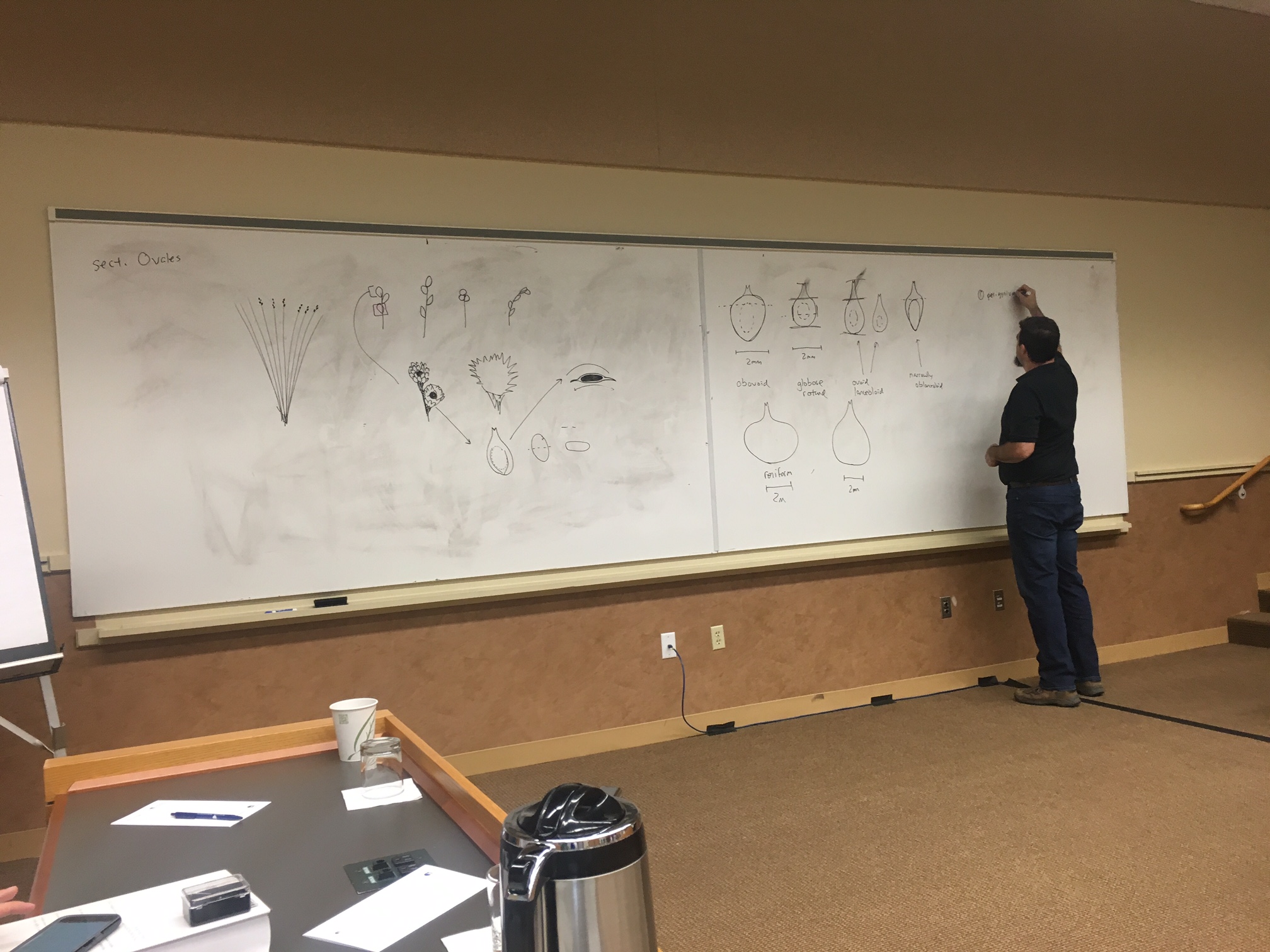
A few weeks ago I attended the 3rd bi-annual (biennial???) Pennsylvania Botany Symposium, an event organized by a number of my colleagues. The first day of the event consisted of several workshops for botanists to learn about particular plant groups. I chose to go to the sedge workshop, as I've lost a lot of my sedge knowledge as I've transitioned from a field biologist to having a greater focus on conservation planning (=more inside time!). My friend Dwayne Estes from Austin Peay State University was the instructor for the class and I've heard great things about his sedge class before.

I really can't say enough good things about the class. Dwayne is an excellent teacher and was really able to convey a lot of knowledge.  This is especially true as he normally teaches this material as a five day class in North Carolina. One thing that was emphasized is the drawing of botanical structures to learn the differences between the different sections of Carex--something that is a lost art among modern taxonomists and is something I definately need to practice.

Creating a Topographic Roughness Index for Pennsylvania

In the development of some data layers for a species distribution modeling project, I determined that one of the environmental drivers we might want to use was a measure of Topographic roughness. The topographic ruggedness index (TRI) appears to have been developed by Riley et al. (1999) to express the amount of elevation difference between adjacent cells of a digital elevation grid.

An excellent post by user ‘whuber’ gives a good workflow for creating a TRI:

Compute s = Focal sum (over 3 x 3 square neighborhoods) of [DEM].
Compute DEM2 = [DEM]*[DEM].
Compute t = Focal sum (over 3 x 3 square neighborhoods) of [DEM2].
Compute r2 = [t] + 9*[DEM2] - 2*[DEM]*[s].
Return r = Sqrt([r2]).

Using this as a guide, I created the a TRI layer in ArcGIS using these steps.

So starting with the standard 30-meter USGS DEM (we’ll call this layer “[DEM]”), we calculate the focal sum (over 3 x 3 square neighborhoods) of [DEM] using the Focal Statistics Tool in ArcGIS.

Next we’ll calculate the square of the DEM, naming it “[DEM2]” using the Square Tool in ArcGIS.

Next we calculate “t” which is the focal sum (over 3 x 3 square neighborhoods) of [DEM2].

I was half tempted to stop here as the map appeared to represent what I was going after for this particular species. But we had to complete the analysis, so we used Raster Calculator to compute  r2 which is equal to the  [t] + 9*[DEM2] – 2*[DEM]*[s].   Then we just take the square root of r2 and get this map, which represents topographic roughness for the state:

The darker the color, the more rough the area is.  This appears to be true in the deep valleys section of northcentral PA, as well as the ridge and valley and lots of the Waynesburg Hills in the SW corner.

Although, we have a high resolution LiDAR-derived DEM for the state, this TRI developed from the 30-m dataset should be good enough for our needs, as the error in the DEM should be negligible especially given the modeling environment. Still, it would be fun to run at the finer scale.